Entry G7: Density and Diameter
Density and diameter give you a feel for how strongly connected the full graph is: whether it’s dense or sparse. To get these measures, I need to calculate three things:
- Number of possible relationships
- Global density
- Diameter
The notebooks where I did my code for this entry can be found on my github page. I created three notebooks, one for each graph model. These notebooks contain the code for Entries G6, G7, and G8.
- Entries G6, G7, G8: Global Metrics Unimodal Graph Model
- Entries G6, G7, G8: Global Metrics Biimodal Graph Model
- Entries G6, G7, G8: Global Metrics Mixed Graph Model
- A notebook with just the global graph density can be found in the Entry 15 notebook
Note, after I created a multigraph with all three graph models, the code changed significantly. You can read Entry 15 for the results of these changes, but that entry is a supplement to this one, not a replacement.
Number of possible relationships
I’m really only interested in this metric due to how it contributes to density. For density, we first need to know the actual number of relationships (calculated in Entry G6) and the number of relationships that are possible for our given graph model.
Keep in mind that the graph model does determine how many relationships are possible.
Unimodal
To calculate this metric for a directed unimodal graph, we multiply the number of nodes (also calculated in Entry G6) by one less than the number of nodes.
Directed unimodal graph:
$pr = n \times (n - 1)$
Since each node in an undirected unimodal graph can only be connected to any other node by a single relationship, we divide the calculation above by 2.
Undirected unimodal graph:
$pr = \frac{n \times (n - 1)}{2}$
Where
- pr = number of possible relationships
- n = node count
For the unimodal graph of the Marvel Universe Social Network (an undirected unimodal graph), with 6,439 nodes, the calculation would look like this: $\frac{\text{6,439} \times \text{6,438}}{2} = \text{20,727,141}$
Bimodal
The bimodal graph has even more options. This is because the graph can be either directed or undirected and it can also limit relationships to only those between different node types or can allow connections between any nodes regardless of node type.
For bimodal graphs that allow relationships between any nodes regardless of type, use the same calculations as the unimodal graphs, paying attention to whether it is directed or undirected.
For bimodal graphs that only allow nodes to connect to nodes of the other type, we simply take into account the number of each type of node. We do this because the number of possible relationships is constrained by the allowed relationships.
Directed bimodal graph:
$pr = (n1 \times n2) \times 2$
Undirected bimodal graph:
$pr = n1 \times n2$
Where
- pr = number of possible relationships
- n1 = node type 1
- n2 = node type 2
For the bimodal graph of the Marvel Universe Social Network, with 6,439 hero nodes and 12,651 comic nodes, the calculation would look like this: $\text{6,439} \times \text{12,651} = \text{81,459,789}$
Notice that while the number of possible relationships is higher than in the unimodal version of our graph, it isn’t as much higher as you may expect considering there are 12,651 more nodes in the bimodal version. This is the result of our constraint only allowing relationships from heroes to comics (and vice versa), but not between heroes or between comics.
If we were to use the same calculation as the undirected unimodal graph, our numbers would look like this: $\frac{\text{19,090} \times \text{19,089}}{2} = \text{182,204,505}$. That’s a little over 100 million more possible relationships in an undirected graph than the correct calculation.
Density
Density tells us what fraction of all possible relationships actually exist. The result will always lie between 0 and 1. Most graphs are sparse, which means they have a low density.
The calculation is:
$d =\frac{r}{pr}$
Where:
- d = density
- r = relationship count
- pr = number of possible relationships
Caution, remember the calculation for the number of possible relationships is different depending on directed/undirected and unimodal/bimodal models.
Diameter
Diameter measures the longest way to get through the graph in the shortest way possible.
Now the longest shortest path is rather confusing, so here are some concrete examples.
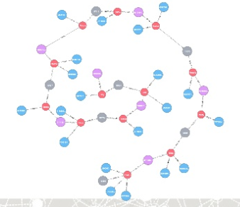
In this example from Max De Marzi’s Fraud Detection slideshare the graph is long and snaking. The shortest path from one end of the graph to the other is 26, i.e., you have to traverse 26 relationships to get from the start node to the end node.

In this example from the cliques caveat in Entry G5, the graph is much more condensed. It only takes 1 relationship traversal to get from any node to any other node regardless of where you start.

As you can see from the second example, you don’t have to touch every node in the graph. You are just looking to see the maximum number of relationships you have to travers to get from a node to another node.
As you may have deduced from the second example, you can’t go through other nodes/relationships to make the diameter bigger. That’s where the shortest part of “longest shortest path” comes in.
So another way of saying this is: what is the maximum number of relationships you have to traverse in the shortest path from a node to another node in the full graph.
