Entry 44: Decision Trees

In entries 35 through 42 we learned how to find linear patterns using Regression algorithms. But what if the patterns in the data aren’t linear? This is where Decision Trees come in. Decision Trees are the foundation for Random Forests, which Hands-On Machine Learning points out on page 175 “are among the most powerful Machine Learning algorithms available today.”

The notebook where I did my code for this entry can be found on my github page in the Entry 44 notebook. Fair warning, it’s pretty messy.

Learning Style

Supervision	Prediction types
Supervised	Regression
	Classification

Description

A Decision Tree is like an automatic if/else creation algorithm. If you’re not familiar with if/else statements yet, Introduction to Machine Learning with Python makes a good analogy on page 72; think of it like a game of 20 questions. By asking “yes/no” or “true/false” questions you can hone in on the correct answer.

A simple example would be figuring out what type of fruit someone is thinking of:

• Question: Is it red?
• Response: Yes
• Question: Is it the diameter of a quarter?
• Response: Yes
• Answer: It’s a cherry

Andreas and Sarah use animal classification as their example in Introduction to Machine Learning with Python and provide a nice visualization in the mglearn package.

Terminology

When looking at a tree like the one above, it’s helpful to know the terms that refer to different parts of the illustration.

Tree

Keep in mind that “tree” doesn’t refer just to the illustration. “Tree” refers to the results of the decision tree algorithm, whether or not those results are visualized as a pretty picture, like the animal classification above, or just text or a list of rules.

However, since it’s easier to understand concepts that can be visualized, I’ll use the illustration above to point out the different parts of a tree. Just keep in mind that ultimately, these terms refer to the concepts that are being visualized.

Node

Each of the boxes is called a node. Each node represents all the data that meets the criteria up to that point.

In English, this means that the node at the top of the illustration, “Has feathers?” holds all the data. The node below it “Can fly?” holds all data where the observation did have feathers while the node “Has fins?” holds all the data where the observation didn’t have feathers.

Root Node

The node at the top of the tree is called the root node. It’s always at the top and always includes all the observations.

Terminal Node or Leaf Node

When there are no more branches off of a node it’s called a terminal node or leaf node (get it? A branch ends in a leaf). The terminal or leaf nodes from the animal classification tree are the ones that are actual animals “Hawk”, “Penguin”, “Dolphin”, and “Bear”.

Child and Parent Nodes

A child node is any node that has a parent node.

The root node, “Has feathers?”, would be an obvious parent node since all nodes originate from that one. The children of “Has feathers?” are “Can fly?” and “Has fins?”. As there is no node that “Has feathers?” comes from, it has no parent.

If we follow the “Can fly?” node, we’ll reach it’s children “Hawk” and “Penguin”, which are also leaf nodes.

Split, Branch, and Test

From the root node, the data is then split into smaller and smaller subgroups based on true/false criteria. The successive splits form branches with more and more limited observations.

Unsurprisingly, this separating process is called spliting and each split is determined by a test. The test is the criteria listed in the node.

An example is “Can fly”: if the data point passes the test because the creature can fly it goes down the “True” split, if it fails the test because the creature can’t fly then it goes down the “False” split.

Edge

The splits are represented by edges, which are the lines that lead to the next set of nodes and have the label “True” or “False” next to them.

Depth

Depth labels the different levels of the nodes and is used to refer to how far down the tree a node is located or how many levels a tree has.

The root node “Has feathers?” is at depth 0, while the leaf node “Hawk” is at depth 2. In programmer language, this means that the depth of the tree is 0 indexed.

Depth is used to control how many splits a decision tree can have. This is usually done by pruning a tree and comes in handy when limiting the complexity of the model.

Prune

To prune a tree is to either stop the splitting based on specific criteria or to remove leaf/child nodes after the tree has been trained. I’ll go into this in depth in Entry 47.

Stump

A stump is a tree that’s been pruned to a depth of 1 and only has one split.

Purpose

Flexibility

Decision trees can find more complex relationships than linear models due to their flexibility.

Machine Learning with Python Cookbook puts it like this on page 233:

Tree based learning algorithms are a broad and popular family of related nonparametric, supervised methods for both classification and regression.

Since I didn’t remember what nonparametric meant, I found a good definition of nonparametric data on Machine Learning Mastery:

data that does not fit a known or well-understood distribution

Hands-On Machine Learning points out on page 181 that Decision Trees are considered nonparametric, not because the number of parameters are unlimited, but because the number of parameters isn’t set prior to training. This brings in the concept of “degrees of freedom,” which you may or may not remember from a statistics class.

As a quick refresher degrees of freedom refer to the number of values of a statistic that are free to vary. Polynomials are a great example of this. The degrees of freedom in $x^2 + 7x + 10$ (degrees of freedom = 3) is much lower than the degrees of freedom in $3x^8 - 6x^7 + 9x^6 - 4x^5 + 2x^3 - x^2 + 7x - 18$ (degrees of freedom = 9).

Due to this freedom, each feature fed to the tree algorithm can be thought of as a term in the polynomial. However, trees can split the same feature in different ways on different branches, allowing a nearly unlimited number of potential degrees of freedom.

For example, in the Titanic dataset the feature “fare” is used multiple times as the test in different splits. Even at a depth of 4, we can see “fare” used at depths 1, 2, and 3 in multiple branches.

Interpretability

Interpretability is one of the major benefits of Decision Trees. Part of this is being able to visualize the tree as a human readable chart. The export_graphviz function from the sklearn.tree module handles this. I go into detail on how to use this function in conjunction with others to either visualize the tree in the Notebook or save to file in Entry 45.

I used the highly simplified example from the mglearn package in the Terminology section, but wanted to include a more realistic preview here along with an explanation of what information it holds.

• The top, unlabeled line in most of the nodes is the threshold used to split the node into the next set of children nodes. Notice that this line is only included in parent nodes. This makes sense because leaf nodes don’t have any splits, thus they don’t have any split criteria.
  • In the root node of the above example petal_length <= 2.45 is the criteria for splitting out the children nodes.
• gini: the impurity measure. If you’re using entropy, this line will be labelled entropy. If you’re using a Regression Decision Tree, the line label will be whatever impurity measure you picked.
  • The impurity of the orange node is 0.0 because all of the samples belong to the virginica class.
• samples: the number of observations in the node.
  • The orange node has 40 observations (out of the total 120 observations) that met the criteria of a petal length less than or equal to 2.45.
  • The purple node has 36 observations that met the criteria of petal length not less than or equal to 2.45 AND petal width not less than or equal to 1.75.
• value: a list with the number of observations in the node that belong to each class.
  • The example diagram uses the Iris dataset and has 3 classes. As such, for the green node value = [0, 39, 5] means that 0 of the samples are in the virginica class, 39 are in the setosa class, and 5 are in the versicolor class.
• class: indicates the majority class of the of the node. If there is a tie in classes, it returns the value first in the list of classes.

Behavior

Decision trees basically use training data to determine if/then statements to create a series of rules to predict an answer. The determination for each split is based on the specific feature that holds the most information about the target variable. To make the prediction, the model then follows the if/then statements until it reaches a final prediction.

Applied Predictive Modeling points out on page 173 that “the if-then statements generated by a tree define a unique route to one terminal node for any sample.” In simpler terms, each observation can follow one and only one path to an answer.

Max and Kjell continue to point out that these statements can be collapsed into a rule: “a set of if-then statements […] that have been collapsed into independent conditions.”

If we use the little mglearn chart as an example, the following would be rules:

• If Has feathers = True & Can fly = True then Hawk
• If Has feathers = True & Can fly = False then Penguin
• If Has feathers = False & Has fins = True then Dolphin
• If Has feathers = False & Has fins = False then Bear

If we translate that into a business case, we could use something like this in the retail industry. If a customer is looking at “Young Adult” books by “female authors” in the “fantasy genre” this person will most likely buy “The Song of the Lioness” series by Tamora Pierce.

If Young Adult = True & author gender = female & fantasy genre = True then Song of the Lioness

Since Tamora Pierce was popular in the 1980s and 1990s, this prediction may be out of date. A more updated prediction would probably be something like “Harry Potter,” but model staleness is a topic for another series of posts.

Using hard coded rules tends to be a first step in programmatically controlling some kind of business process. Creating these kinds of rules is generally time consuming and keeping them current is challenging. Decision trees could be used to replace such manual systems or streamline the process if hard coded rules are necessary.

This is all well and good, but how does the model choose which features to use at each split?

The main idea is that the model looks for the feature with the most signal, also known as having the highest information gain. That’s a little oblique, so let’s use the Iris dataset as an example. There are four features:

• Sepal length
• Sepal width
• Petal length
• Petal width

Creating a pairplot of the four features with the species as the color, we can see how different combinations of features compare to each other. But how do we decide which single feature is the most impactful?

Impurity Measures

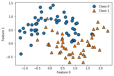
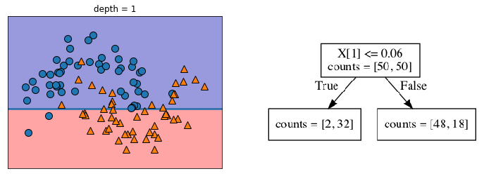
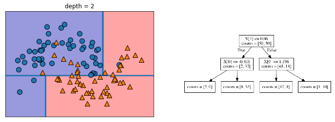
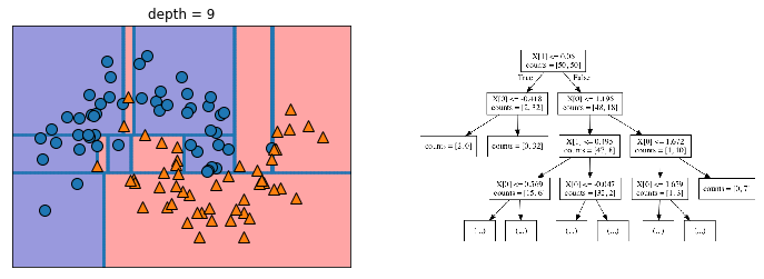
The way the model finds the feature with the highest signal is to use an impurity measure. This measure attempts to find the best split that separates the classes the most cleanly. I’ll go into impurity measures in detail in Entry 48, but the mglearn package has a great illustration of the successive splits that a decision tree could makes to illustrate the main idea.

Introduction to Machine Learning with Python explains the succession of splits nicely on page 75:

You can think of each test as splitting the part of the data that is currently being considered along one axis.

As can been seen above, this process essentially breaks the data into boxes that contain similar observations. However, as can be seen in the last chart of the series above, these boxes can be less helpful when they only contains 1-3 data points and become isolated among clusters of dissimilar data points.

We can see an example of this in the narrow blue strip in the upper right quarter among an otherwise homogeneous orange section. There is also a narrow orange strip in the blue section in the upper left, with two small boxes under it that include only a single point in each box.

As demonstrated by the illustration above, narrowing the data to this small of a subsample results in 100% accuracy on the training data, but doesn’t generalize well to data it has never seen. In other words, the model is prone to overfitting. If you need a refresher, overfitting is discussed in Entries 17 and 30. I’ll also be going into overfitting, underfitting, and data sensitivity in Entry 46.

The other limitation of using impurity is that while it results in the best split at that particular depth, it doesn’t necessary result in the best splits for the overall data. Hands-On Machine Learning puts it nicely on page 180:

the CART algorithm is a greedy algorithm: it greedily searches for an optimum split at the top level, then repeats the process at each subsequent level. It does not check whether or not the split will lead to the lowest possibly impurity several levels down. A greedy algorithm often produces a solution that’s reasonably good but not guaranteed to be optimal.

Finding the “optimal” solution, the one that has the lowest possible impurity as the end result is considered an NP-hard problem, which is currently unsolvable. So while this is a limitation, it still produces very good results.

Subcategories

I’ll talk more about subcategories in Entry 50, but here’s a list for now:

• ID3
  • Nodes can have more than 2 child nodes
• C4.5 and C5.0
• CART
  • Produces binary trees, i.e. each node only produces 2 child nodes
• CHAID
• Decision Stump
• Conditional Inference Trees
• GUIDE

Parameters

A full list of parameters can be found on the Scikit Learn pages sklearn.tree.DecisionTreeClassifier and sklearn.tree.DecisionTreeRegressor, but the ones I use in the Notebooks include:

• criterion: The function to measure the quality of a split.
• max_depth: The maximum depth of the tree. Limits the depth of all branches to the same number.
• min_samples_split: The minimum number of samples required to split an internal node.
• min_samples_leaf: The minimum number of samples required to be at a leaf node.
• max_leaf_nodes: Grow a tree with max_leaf_nodes in best-first fashion. Best nodes are defined as relative reduction in impurity.
• min_impurity_decrease: A node will be split if this split induces a decrease of the impurity greater than or equal to this value.
• min_impurity_split: Threshold for early stopping in tree growth. A node will split if its impurity is above the threshold, otherwise it is a leaf.

Strengths

• Highly interpretable (white box models)
• Can find nonparametric patterns
• Can make regression, classification, or multioutput predictions
• Can handle many types of predictors (sparse, skewed, continuous, categorical, etc) Applied Predictive Modeling page 174
• Requires minimal data preparation
• Handles missing values
• Doesn’t require centering, scaling, or normalization
• Can generate rules, which can be pruned and hard coded
• Automatically handles feature selection

Missing data

Applied Predictive Modeling has a nice explanation on page 180 about how decision trees handle missing data:

When building a tree, missing data are ignored. For each split, a variety of alternatives (called surrogate splits) are evaluated. A surrogate split is one whose results are similar to the original split actually used in the tree. If a surrogate split approximates the original split well, it can be used when the predictor data associated with the original split are not available. In practice, several surrogate splits may be saved for any particular split in the tree.

Limitations

• Prone to overfitting
• sklearn.tree.DecisionTreeRegressor and other tree-based regression models, are not able to extrapolate; i.e. they can’t make predictions outside the range of the training data. Introduction to Machine Learning with Python page 82
• Model instability (sensitive to small variations in the training data)
• If features are highly correlated, more features may be selected than necessary Applied Predictive Modeling page 181
• The sklearn implementation ignores features with missing values

Up Next

Visualizing Decision Trees

Resources

• Hands-On Machine Learning with Scikit-Learn, Keras, and TensorFlow
• Introduction to Machine Learning with Python
• Machine Learning with Python Cookbook
• Applied Predictive Modeling
• Python Data Science Handbook
• A Gentle Introduction to Nonparametric Statistics
• Degrees of freedom (statistics)
• 1.10. Decision Trees
• sklearn.tree.DecisionTreeClassifier
• sklearn.tree.DecisionTreeRegressor
• 1.10.6. Tree algorithms: ID3, C4.5, C5.0 and CART
• chefboost
• C4.5
• decision-tree
• Decision Trees - An Introduction