Entry 35: Regression

8 minute read

Regression is used to predict on continuous data, for example housing prices. Logistic Regression is the subcategory that is the exception, as it does classification only.

Scikit-Learn has parameters that allow several of the subcategories of regression, such as Ridge, Lasso, and Elastic Net, to handle both regression and classification.

The notebooks where I did my code for this entry can be found on my github page:

Learning Style

Supervision	Prediction types
Supervised	Regression
	Classification

Description

The gist of regression is that it uses a linear function to fit the data. For the simplest cases, it’s just like the equation for a line:

y = mx + b

Where:

y = y
m = slope of the line
x = x
b = y-intercept

Wave line

To account for more than one input, the full equation for linear regression is a little more complicated.

The equation as listed on page 47 of Introduction to Machine Learning with Python is:

$\hat{y} = w_{0} x_{0} + w_{1} x_{1} + \dotsb + w_{p} x_{p} + b$

Where each x represents a feature (just like in the single variable version where x is the input and y is the output) and w is a learned weight for each feature. The text continues, and points out that the equation for a single feature is:

$\hat{y} = w_{0} x_{0} + b$

This equation is exactly the same as the one for a line above, except $w_{0}$ has been substituted for m. A simplified way of thinking about this would be that the slope (m) is calculated for each feature and used as the weight (w). Introduction to Machine Learning with Python puts it like this:

For more features, w contains the slopes along each feature axis. Alternatively, you can think of the predicted response as being a weighted sum of the input features, with weights (which can be negative) given by the entries of w.

It expounds further on page 48:

Linear models for regression can be characterized as regression models for which the prediction is a line for a single feature, a plane when using two features, or a hyperplane in higher dimensions.

Subcategories

So, all of that is well and good, but how are the weights/theta values calculated? According to Introduction to Machine Learning with Python on page 49, the way the model learns the weights and how it controls complexity are the differentiating factors between the various subcategories of regression. These subcategories are:

Ordinary Least Squares (OLS)
- Normal Equation
- Gradient Descent
Ridge Regression
Lasso Regression
Elastic Net
Logistic Regression

Each subcategory will have its own entry explaining how it differs from the others.

Purpose

The purpose of regression is to find the best fit “line” for the feature space and then apply that to data points that haven’t been seen before to predict the output of the new data. The way this is implemented is via linear algebra using a vectorized version of the equation.

Vectorized equation

The equation for linear regression as listed on page 112 of Hands-On Machine Learning with Scikit-Learn looks a little different than the one in Introduction to Machine Learning with Python:

$\hat{y} = \theta_{0} + \theta_{1} x_{1} + \theta_{2} x_{2} + \dotsb + \theta_{n} x_{n}$

However, all the changes are superficial:

b is moved to the front of the equation and written as $\theta_{0}$
The ws are written as $\theta$s
The unknown number of elements is written as n instead of p
The subscripts for the xs starts at 1 instead of 0

The nice thing about the slight alterations to the equation is that it makes it easier to understand the vectorized representation of the equation (from page 113 of Hands on Machine Learning with Scikit-Learn):

$\hat{y} = h_{0}(x) = \theta x$

Where

$\theta$ is a vector (i.e. list) of weights, with the first value being the y-intercept type value (represented by b in Introduction to Machine Learning)
x is the matrix of feature values (i.e. the DataFrame) with the first column ($x_{0}$, not listed in the equation) being all 1s so that $\theta_{0}$ is always evaluated as the same value

As an example, I created a fake theta array for a subset of the planet data. The first value in the theta array (6.5) is b in Introduction to Machine Learning with Python and $\theta_{0}$ in Hands-On Machine Learning with Scikit-Learn. The rest of the values are the weights for each feature (the ws in Introduction to Machine Learning with Python and $\theta_{1}$ through $\theta_{n}$ in Hands-On Machine Learning with Scikit-Learn.

theta = pd.Series([6.5, 2.5, 8.1, 0.3, 1.7, 3.8, 5.9])
theta

  6.5
  2.5
  8.1
  0.3
  1.7
  3.8
  5.9
dtype: float64

The subset of planet data, along with the initial column of 1s (remember the first column needs to be all 1s so that $\theta_{0}$ remains the same value) looks like this:

	theta0	mass_1024kg	diameter_km	mean_radius_km	density_kg_m3	gravity_m_s2	escape_vel_km_s
0	1	0.3300	4879.0	2439.4000	5427	3.7	4.3
1	1	4.8700	12104.0	6051.8000	5243	8.9	10.4
2	1	5.9700	12756.0	6371.0084	5514	9.8	11.2
3	1	0.0730	3475.0	1737.4000	3340	1.6	2.4
4	1	0.6420	6792.0	3389.5000	3933	3.7	5.0
5	1	1898.0000	142984.0	69911.0000	1326	23.1	59.5
6	1	568.0000	120536.0	58232.0000	687	9.0	35.5
7	1	0.1260	5149.4	2574.7000	1882	1.4	2.6
8	1	86.8000	51118.0	25362.0000	1271	8.7	21.3
9	1	102.0000	49528.0	24622.0000	1638	11.0	23.5
10	1	0.0146	2370.0	1188.3000	2095	0.7	1.3

The dot product is then calculated for the theta array and the planet feature values to give the linear regression output.

planet_df.values.dot(theta)

array([  49524.37497204,  108884.89493742,  114733.44748931,
         34373.64250797,   62769.81500023, 1186588.23000145,
        996649.25      ,   45709.42419369,  424207.3300024 ,
        411789.95      ,   23131.85651432])

For more information on linear algebra/matrix multiplication and linear regression, see weeks 1 and 2 of Andrew Ng’s Machine Learning course on coursera.org. For information on how to implement it in a machine learning context, see the note in Hands-On Machine Learning with Scikit-Learn on page 113 (mainly when and why $\theta$ needs to be transposed).

Behavior

Single feature

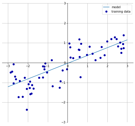
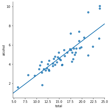
The line for a single feature is easily visualized, just as in the first chart at the beginning of the entry, which uses the synthetic Wave dataset created for the book. Another example can be seen using the car_crashes sample dataset in Seaborn:

Wave line

Two Features

The plane for two features is also easily visualized in a 3D visualization.

The concept of a plane is easily seen in this chart from the blog Machine Learning in Action during a discussion of SVMs.

Taking this concept and applying it to data in a plane (instead of separated by a plane like the SVM based example above), I created a visualization based on the planet dataset I originally started this data science journaling journey with. Remember how the data didn’t meet the criteria of independently and indentically distributed? Well, now that works in my favor because I know exactly which features should be correlated and the mathematical way in which they’re related.

For data that should show on a plane, I needed a feature that depended on two other variables. My options were:

density = $\frac{M}{v}$
gravity = $\frac{GM}{r^2}$
escape velocity = $\sqrt{\frac{2GM}{r}}$

Where:

M = mass
v = volume
G = gravational constant
r = radius

Of the three, density had the most obvious example:

Density chart

The color saturation of the dot indicates how close it is to the viewer (darker is closer, lighter is farther away). In this particular configuration, the data points almost seem to form a line (except one data point, which stands above the line). However, the darkess of the dots reveals that they vary along the near/far axis. As such, it appears they all (except one) fall along the same plane.

More than Three Features

As the number of dimensions goes up, it becomes more and more difficult to visualize and conceptualize.

Parameters

Depend on which subcategory of regression is being used. This will be populated in the entry for each specific subcategory.

Strengths

Fast to train
Fast to predict
Easily scale to very large datasets
Work well with sparse data
Easy to intrepret / easy to see feature importance
Performs well when the number of features is large compared to the number of observations (ex, 104 features but only 5 observations)

Limitations

In low dimensions, linear models appear to have very limited usefulness. However, as more dimensions are added, the model becomes more powerful and can become overfit
Often unclear why coefficients are the what they are, particularly if there are highly correlated features
Specializes in linear relationships
- While features can be augmented to help capture curvilinear relationships (like quadratic or cubic), Linear Regression may not adequately capture nonlinear relationships
- Adding additional features to augment curvilinear relationships can create or exacerbate model overfitting
As it uses the mean of the residuals, it is susceptible to outliers
May become erratic when the number of predictors is higher than the number of observations (ex, 14 features but only 5 observations)

Evaluation

The appropriate metrics depend on whether the model is being used for regression or classification. Discussions on the available metrics can be found in prior entries:

Datasets

Appropriate datasets depend on whether the model is being used for regression or classification. Some same datasets include:

Resources

Up Next

Ordinary Least Squares (OLS)

Twitter Facebook LinkedIn

Julie Fisher