
Entry 15: Categorical Correlation/Collinearity
To ensure my process worked, I used it on multiple datasets. The code from notebook to notebook is mostly the same, just run on different data. Per usual, the notebooks can be found on my github page:
- Entry 15a notebook (Mushroom)
- Entry 15b notebook (Solar Flare)
- Entry 15c notebook (Nursery)
- Entry 15d notebook (Chess
The Problem
Correlation and collinearity calculations tend to rely on numeric values or at the very least, ordinal categories where the order in which they are placed have some kind of meaning. A simple example of the kinds of challenges introduced with unordered categorical variables can be seen in the bike share dataset.
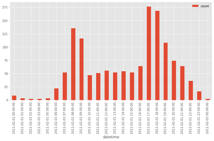
When looking at the count of bikes used in an hour, there is a clear relationship between time of day and the number of bikes shared. Most prominent are the spikes around the start and end of the work day.
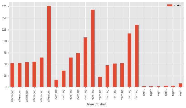
When these same values are reordered by category - like morning, evening, and night - the patterns that were obvious before become obscured. And if we sort the values differently (below has a secondary sort on ‘count’), it could seem like there are different relationships. The secondary sort on count gives the impression of escalation across the values. But if it had a random secondary count, there probably wouldn’t be any discernible pattern.
When the categories aren’t ordinal, doing mathematics on them becomes arbitrary and subjective - how would you subtract California from the average of states? What would the average of states even be? Kansas?
The Options
Encode and use correlation
I could one-hot encode the values first, then run correlation. This quickly becomes unwieldy. The 22 features of the Mushroom Dataset for example turn into 112 one-hot encoded features.
Cramer’s V
Cramer’s V is based on a nominal variation of Pearson’s Chi-Square Test. It has a range of [0,1], where 0 means no association and 1 is full association (no negative values, either there is an association or there isn’t). Like correlation, it is symmetrical (the diagonal divides mirror images of the two sides).
Theil’s U / Uncertainty Coefficient
Because Cramer’s V is symmetrical, there is the potential for information loss. Shaked Zychlinski provided the following illustration of this problem in The Search for Categorical Correlation:
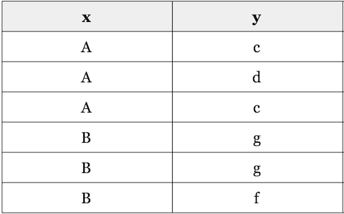
If I know x I can’t predict y with any certainty. However, if I know y, then I can accurately determine the value of x.
Per Shaked, Theil’s U is “based on the conditional entropy between x and y — or in human language, given the value of x, how many possible states does y have, and how often do they occur.”
The range of values is the same as Cramer’s V: [0,1], where 0 means no association and 1 is full association.
The Proposed Solution
I visualized the Spearman and Pearson correlations for all categorical encodings available via the category-encoder package. This was partly a continuation/combination of the correlation exploration from Entry 7 and the categorical encodings from entry Entry 14. This also gave me something to compare to the Cramer’s V and Theil’s U methods.
I ran the above on four datasets:
- Mushroom Dataset
- Observations: 8,124
- Attributes: 22
- Solar Flare Dataset
- Observations: 1,389
- Attributes: 10
- Nursery Dataset
- Observations: 12,960
- Attributes: 8
- Chess Dataset
- Observations: 3,196
- Attributes: 36
Expanded feature sets
In the Mushroom dataset, most of the correlation methods found gill attachment and veil color as correlated. When the categorical features get expanded out to one feature per category (i.e. a color column turns into one column each for red, blue, green, etc) it gets difficult to tell if a column should be removed for collinearity. If a single category is correlated to another single category, should one full attribute be removed from the dataset? Just one of the categories?
Mathematical relationships
I’m also not sure how well algorithms are at finding relationships between features. For example, when I was playing with the planet dataset I realized that five of the features are mathematically related. With mass, radius, volume, density, and gravity if you have any two of the values you can calculate the remaining three. Would a machine learning algorithm be able to detect and use these mathematical formulas? The assumption that the features are independent and identically distributed (discussed in Entry 10) lead me to believe that such relationships would mess up or confuse the algorithms. It’s a question for another day.
Correlation methods
It was interesting to see the differences between the Pearson and Spearman correlations in the different datasets. For example, in the Mushroom dataset, they find almost the exact same correlations with the JamesSteinEncoder, but Spearman finds negative correlations that Spearman doesn’t with the LeaveOneOutEncoder. The CatBoostEncoder also returned different results than the other encoding methods on at least two of the datasets.
Overall for this first analysis, I liked the Theil’s U best. Theil’s U and Cramer’s V both made if very clear which categorical features were correlated, but Theil’s U also indicated which of the two features should be kept.
The Fail
I detoured a bit when visualizing each of the categorical encodings by Pearson and Spearman correlation measures. The detour did give me a much better understanding of the category-encoders package. For example, the encoding methods break down into two main categories:
- Target independent (the encoding method is not related to the attribute being predicted)
OrdinalEncoderOneHotEncoderBinaryEncoderHashingEncoderBackwardDifferenceEncoderHelmertEncoderPolynomialEncoderSumEncoder
- Target dependent (i.e. target encoded, where the encoding method is based in some way on the attribute being predicted)
CatBoostEncoderJamesSteinEncoderLeaveOneOutEncoderMEstimateEncoder(likelihood - logistic predictions) andTargetEncoder(continuous variable - regression predictions)WOEEncoder
The inconsistent results returned by the CatBoostEncoder will need to be explored more later. I’ll also need to look into the questions raised in the Proposed Solution section: how do the algorithms understand a feature when it is expanded out and can the algorithms find and use mathematical relationships across multiple features.
The detour into Pearson and Spearman correlations also allowed me to develop a function to remove undifferentiated columns (the same value for every observation). Because every value is the same, these columns don’t contribute to correctly predicting the target variable. In addition, correlations return errors (result is NA, which can’t have further calculations run and can’t be visualized) for these values.
Up Next
Resources
The major resource for this entry was The Search for Categorical Correlation.